Chapter 5. Measurement
Prev		Next

Chapter 5. Measurement

Table of Contents

5.1. Sensor Configuration

5.1.1. Difference between Sensors, Channels, and Evaluations
5.1.2. Sensor Helper
5.1.3. Order of Sensors and Evaluations
5.1.4. RS-485 Serial Interface

In the Measurement → Sensors menu, sensors can be added and basic parameters can be configured by using the Sensor Helper (see Section 5.1.2, “Sensor Helper”). After having configured the sensors, two buttons are available for each sensor: Delete and Change. These allow a user to delete or change an existing sensor with help of the Sensor Helper.

Figure 5.1. Sensor Definitions

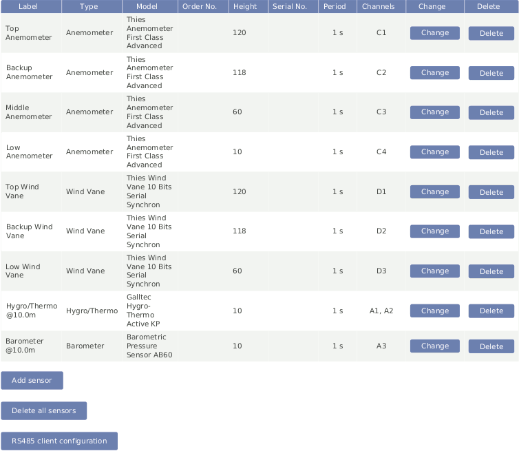
Screenshot of the Sensor Definitions Page

Below the sensor definitions overview you can find four buttons: Add sensor, Delete all sensors, RS-485 serial interface and Download sensor database.

Add sensor:: Opens the Sensor Helper to configure a new sensor.
Delete all sensors: If all sensors should be deleted, e.g. after a completed measurement campaign, you can click on Delete all sensors to remove all sensors from the configuration in one step.
RS-485 serial interface: Occasionally it can be necessary to send a command to a sensor connected to an RS-485 client port, e.g. in order to examine communication problems or to change sensor's configuration (see Section 5.1.4, “RS-485 Serial Interface”).
Download sensor database: Download a CSV file which describes all the sensors available in Sensor Helper.

	Note
	By clicking on a column headline in the sensor definitions overview, you can sort the selected column in ascending or descending order.

Note

When adding a new sensor or changing the electrical channel of a sensor, recording is stopped automatically. That way, it is clear which measurements use the old configuration and which measurements use the new one. Also, if no sensors at all are configured, recording is switched off. Afterwards, one can switch on recording. Also, recording will be switched on automatically after 20 minutes of no further configuration changes.

	Important
	For some estimations related to solar sensors, the location of the measurement station has to be added in the System → Administration menu (see also Section 4.2, “System Administration”).

	Warning
	Adding or deleting a sensor switches the recording off. The new configuration is unsaved! By clicking on Switch on, the configuration will be automatically saved and recording will resume.

5.1.1. Difference between Sensors, Channels, and Evaluations

To have a better understanding of the sensor management, it is important to know the difference between sensors, channels, and evaluations.

In general, a sensor is an electromechanical device, which records physical values. The physical values are transformed into an electrical value by the sensor. For example, wind speed can be transformed into a frequency. To map these electrical values on the corresponding physical values, an evaluation process has to be performed.

A sensor may be connected to more than one electrical channel of Meteo-42. The number of used electrical channels depends on the kind of sensor and also on the kind of electrical wiring of the sensor. For example, wind vane POT (potentiometer) may use the two analog channels A1 and A2. Another example is the pyranometer Delta-T SN1 that emits two analog voltage signals and one digital status signal. The two analog output signals have to be connected to two analog voltage channels and the digital status signal has to be connected to one digital input.

The evaluation process of the measured values is done by the software of the Meteo-42 data logger. Both pieces of data are saved: the measured physical value at every channel and the evaluated value. Some typical formulas are displayed below.

Most anemometers deliver a rectangle pulse output signal with a frequency proportional to the instant speed. Connecting it to a counter input (i.e. C1 to C12), its frequency will be measured. For the evaluation of wind speed a linear formula will be applied using slope and offset values given in the configuration of the Measurement → Sensors menu.

Equation 5.1. Linear Equation for Wind Speed

v_wind = slope × Cx + offset : Cx > 0; v_wind = minimal_value : Cx = 0

A counter value of 0 results in an output equal to the minimal_value instead of the offset. The offset is ignored in that case. Leaving the minimal_value field blank is equivalent to setting it equal to the offset.

The output signal of many pyranometers is an analog voltage. To measure and record this signal, the output of the pyranometer should be connected to an analog voltage input (i.e. A1 to A12). To interpret the value of the apparent solar radiation, the measured value is internally divided by the specific sensitivity of this sensor. In this case sensitivity has to be configured.

5.1.2. Sensor Helper

In order to simplify the configuration of sensors, Meteo-42 provides a Sensor Helper in the Measurement → Sensors menu. The Sensor Helper guides you through the sensor configuration. It will appear when you attempt to Add sensor or Change a sensor, a channel or an evaluation.

You can select a sensor model by entering a text search query. The search is performed over the sensor type, model name, input channel name, order number and RS-485 protocol type. You can also browse all models by selecting a sensor type and supported model.

Once you select the sensor, the appropriate channel settings will be automatically selected as shown in Figure 5.2, “Sensor Helper with Sensor Settings”. Depending on the sensor, further settings can be configured by the user, e.g. Slope, Offset, Sensitivity, measurement rate, channel, etc..

	Important
	If the sensor doesn't appear in the list of preconfigured sensor, you can always use a generic sensor from the Other Sensor list.

	Note
	Only channels and switches which are not already used by other sensors are available.

Figure 5.2. Sensor Helper with Sensor Settings

Screenshot of the Sensor Helper (default sensor settings)

	Important
	For many sensors, slope and offset values are preconfigured according to the manufacturer's information. Carefully check the values. If calibrated sensors are installed, use the slope and offset or sensitivity values indicated in the calibration protocol of the sensor.

5.1.3. Order of Sensors and Evaluations

The order of sensors and evaluations in the web interface and the LC display is always consistent.

Sensors are ordered by

sensor type (anemometers, wind vanes, thermo/hygro sensors, barometers, precipitation sensors, solar sensors, ultrasonics, power meters, other sensors),
height (from highest to lowest),
and finally the textual label (alphabetically).

Evaluations are ordered by

evaluation type (wind speed, wind direction, humidity, temperature, differential temperature, air pressure, air density, etc.),
height of the corresponding sensor (from highest to lowest),
and finally the textual label (alphabetically).

5.1.4. RS-485 Serial Interface

During the installation process or when changing any sensor settings during deployment, it can be useful to send a special command to a connected RS-485 sensor.

Figure 5.3. RS-485 Serial Interface

Screenshot of the RS-485 Serial Interface

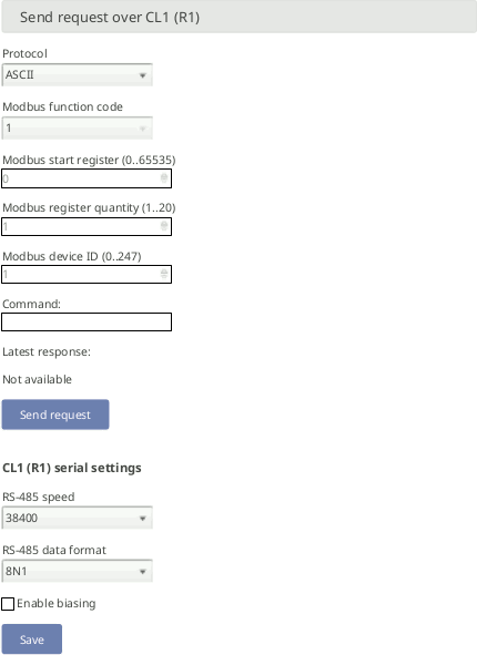
First of all, the general serial settings of the RS-485 client have to be configured according to the configuration of the sensor. All sensors on a RS-485 bus will share the configured settings.

Meteo-42 provides an internal biasing on RS-485 CL1 and CL2. In order to avoid an unnecessary power consumption, the internal biasing can only be enabled if a sensor is already configured on that bus. See Section 11.6, “Connecting Sensors to RS-485 Client” for more information.

Four different protocols are supported: ASCII, Modbus RTU Helper, Modbus RTU and Hexadecimal.

If ASCII protocol is selected, the custom command must be typed by the user in the command box. The following escape sequences representations are recognized for the ASCII commands:

Table 5.1. ASCII escape sequences for RS-485 Serial Interface

Escape Sequence	Symbol
<CR>	U+000D Carriage Return
<LF>	U+000A End of Line
<STX>	U+0002 Start of Text
<ETX>	U+0003 End of Text

If Modbus RTU Helper protocol is selected, the telegram will be automatically composed according to the configured parameters. Press the Send request button to compose and send the command. The command will be displayed in the command box. The required parameters for Modbus RTU Helper frames are: Modbus Function code (1 to 6 supported), Start register (PDU addressing, first reference is 0) and Quantity (quantity of registers/inputs for read only function codes 1 to 4) or Value (for writing function codes 5 and 6), Modbus device ID for the unique sensor identifier in the bus (0..247).

Table 5.2. Modbus RTU function codes supported by Modbus RTU Helper mode for RS-485 Serial Interface

Modbus function code	Description
1	Read coils
2	Read discrete inputs
3	Read holding registers
4	Read input registers
5	Write single coil
6	Write single register

If Modbus RTU protocol is selected, any Modbus RTU frame can be introduced in the command box, e.g. function code 16 which is not supported by the Modbus RTU Helper mode . The frame will not be sent if the Modbus Cyclic Redundancy Check (CRC) is incorrect.

If Hexadecimal mode is selected, any hexadecimal string can be sent.

The communication will be reflected in the logbook including a timestamp. Example of ASCII communication: "RS-485 Request: '01TR00003<CR>', Response: '<STX>000.1 096 +24.6 M 0E*1D<CR><ETX>'". Example of Modbus communication: "RS-485 Request: '0104277400063aa6', Response: '01040c41375c2942c0000041e800006d3d'".

	Note
	The RS-485 serial interface is only available for Admin.

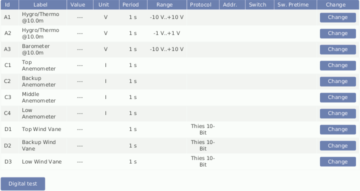
5.2. Measurement Channels

In the Measurement → Channels menu a table is shown, which displays all connected channels with details such as label, value, rate, range, protocol and selected switch. To modify sensor settings, click on Change to open the Sensor Helper (see also Section 5.1.2, “Sensor Helper”).

Figure 5.4. Measurement Channels Overview

Screenshot of the Measurement Channels mask.

	Note
	Click on a column headline in the measurement channels overview to sort the selected column in ascending or descending order.

5.3. Configuring the Evaluation

5.3.1. Evaluation Helper

In the Measurement → Evaluation menu the settings for data evaluation are shown. A table displays the configured sensors with their measured and estimated values. The order of evaluations is explained in Section 5.1.3, “Order of Sensors and Evaluations”. If the settings should be modified, click on Change to open the Sensor Helper (see also Section 5.1.2, “Sensor Helper”).

Figure 5.5. Screenshot of the Configuration for the Evaluation

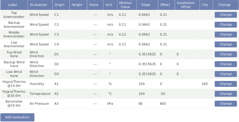
Screenshot of the Evaluation Configuration

In addition to the automatically generated evaluations, it is possible to apply formulas to the measured values or even combine evaluations. The new evaluations can be added in the Evaluation Helper by clicking on Add evaluation. See Section 5.3.1, “Evaluation Helper”.

	Note
	Click on a column headline in the evaluation configuration overview to sort the selected column in ascending or descending order.

5.3.1. Evaluation Helper

The Evaluation Helper introduces a higher flexibility to Meteo-42 sensors configuration. Apart from the automatically configured evaluations which appear when you add a sensor, this tool allows you to generate new evaluations, combining the existing ones by means of a formula. The standard statistics are available for the new evaluation and will be included in the CSV statistics file. The Evaluation Helper also provides some special statistics like the covariance, kurtosis, turbulence intensity or Obukhov length. To use this feature, click Add evaluation in the Measurement → Evaluation menu. The Evaluation Helper will guide you through the configuration process. After choosing a formula from the list, the corresponding parameters will be shown for selection.

	Important
	Only the measured values are saved by default to the CSV statistics file. Estimated values are for information purposes. In order to include estimated values in the CSV statistics file, select the values over the statistics selection interface in the Data → Statistics menu under Select statistics.

5.3.1.1. Addition

Addition of two or three previously configured evaluations.

Equation 5.2. Addition of two elements

A = B + C

Equation 5.3. Addition of three elements

A = B + C + D

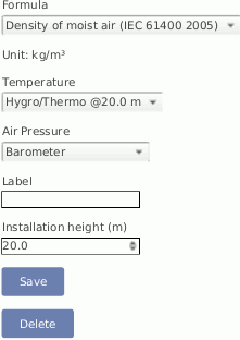
5.3.1.2. Density of moist air

According to IEC 61400-12-1 it is required to measure air density, which is calculated from air temperature and air pressure. Air density has a significant influence on the wind energy calculation. See calculation of wind energy in Section 10.1, “Sensors for Wind Resource Assessment and Wind Farm Monitoring”.

At high temperatures measuring relative air humidity is recommended according to IEC 61400-12-1. In order to calculated density of moist air, Meteo-42 offers two options: with or without relative humidity.

If air density should be calculated without humidity, choose only a temperature and a barometric pressure sensor from the list in the Evaluation Helper (see Section 5.3.1, “Evaluation Helper”). Meteo-42 calculates air density for evaluation with original 1-sec measurement data according to the following formula:

Equation 5.4. Calculation of Density [ρ] of Dry Air

ρ = p / (R₀ × T)

where p is the air pressure, T the air temperature and R_O the gas constant of dry air 287.05[J/kgK].

If relative humidity should be considered for air density calculation, choose also a humidity sensor from the list in the Evaluation Helper (see Section 5.3.1, “Evaluation Helper”). With selected humidity sensor, Meteo-42 calculates density of moist air for evaluation with original 1-sec measurement data according to the following formula:

Equation 5.5. Calculation of Density [ρ] of Moist Air

ρ = 1/T (p/R₀ - RH × p_H₂O (1/R₀ - 1/R_H₂O))

where T is the air temperature, p the air pressure, R₀ the gas constant of dry air 287.05[J/kgK], R_H₂O the gas constant of water vapour 461.5[J/kgK], p_H₂O the vapour pressure, RH the relative humidity.

Figure 5.6. Evaluation for Air Density

Screenshot of the Evaluation Configuration for Air Density

5.3.1.3. Albedo

Surface albedo is defined as the ratio of irradiance reflected to the irradiance received by a surface. It is dimensionless and measured on a scale from 0 (corresponding to a black body that absorbs all incident radiation) to 1 (corresponding to a body that reflects all incident radiation). If an upper pyranometer reading, a lower pyranometer reading, or both is/are less than 2 W/m², the albedo value is invalid.

Equation 5.6. Albedo

Albedo = Reflected Irradiance (W/m²) / Global Irradiance (W/m²)

5.3.1.4. Ampere meter

Based on Ohm's law, you can use the Ampere meter formula to transform the measured voltage to the corresponding current, after introducing the value of the shunt resistor used. This formula can be used with any existing voltage evaluation (e.g. if you previously configured a Gantner A3.1 module).

Equation 5.7. Ohm's law

I = V / R

where I is the current through the conductor in units of amperes, V is the voltage measured across the conductor in units of volts, and R is the resistance of the conductor in units of ohms.

5.3.1.5. Differential temperature

By selecting Differential temperature in the Evaluation Helper, the difference between two temperature measurements can be recorded every second. Choose two temperature sensors from the list for theta 1 and theta 2. According to the following equation the difference is calculated.

Equation 5.8. Calculation of the Temperature Difference [Δtheta]

Δϑ_[K] = ϑ1_[°C] - ϑ2_[°C]

5.3.1.6. Division

Division of two previously configured evaluations.

Equation 5.9. Division

A = B / C

5.3.1.7. Effective irradiance

Effective irradiance (E_eff) in W/m² is the total plane of array (POA) irradiance adjusted for angle of incidence losses, soiling, and spectral mismatch. In a general sense it can be thought of as the irradiance that is “available” to the PV array for power conversion.

Equation 5.10. Calculation of effective irradiance

E_eff = G₀ x I_SC × (1 - α_{I_SC} × (T - T₀)) / I_SC₀

where G₀ : reference condition irradiance (W/m²), I_SC : measured short circuit current (A), I_SC₀ : short circuit current at reference condition (A), T : measured surface temperature (°C), T₀ : surface temperature at reference condition (°C), α_{I_SC} : temperature coefficient of short circuit current (%/°C).

5.3.1.8. Soiling ratio I_SC index

The soiling ratio I_SC index (SR I_SC) is a standard metric for the effects of soiling on energy production. This dimensionless factor is in range 1.0 to 0 and equals 1 when both modules are clean.

Equation 5.11. Calculation of SR I_SC normalized according to IEC 61724-1

SR I_SC = I_{SC_Soiled} / I_{SC_{Soiled^Expected}}

Equation 5.12. Expected I_SC from the soiled device according to IEC 61724-1

I_{SC_{Soiled^Expected}} = E_eff / G₀ x (I_SC₀ ^Corrected / (1 - α_{I_SC} x (T_Soiled - T₀))

where E_eff: effective irradiance at the clean device (W/m²), G₀ : reference condition irradiance (W/m²), I_SC₀^Corrected : corrected reference short-circuit current (A) (see Section 10.19.2, “Ammonit Soiling Measurement Kit SD2100”), T_Soiled : soiled device measured surface temperature (°C), T₀ : surface temperature at reference condition (°C), α_{I_SC} : temperature coefficient of short circuit current (%/°C).

For identical soiled an clean devices, SR I_SC can be calculated as follows (legacy systems).

Equation 5.13. Calculation of SR I_SC for identical soiled and clean devices

SR I_sc = (I_{SC_Soiled} × (1 - α_{I_SC} × (T_Soiled - T₀))) / (I_{SC_Clean} × (1 - α_{I_SC} × (T_Clean - T₀)))

where I_SC is the measured short-circuit current of the soiled and clean modules and T is the measured temperature of the soiled and clean modules respectively.

5.3.1.9. Soiling loss index

The soiling loss index (SLI) is a standard metric for the effects of soiling on energy production. It can be calculated from the effective irradiances of a clean reference panel and a dirty test panel.

Equation 5.14. Calculation of SLI

SLI = (1 - E_{eff_Soiled} / E_{eff_Clean}) × 100

where E_{eff_Clean}: effective irradiance of the clean PV module and E_{eff_Soiled} : effective irradiance of the soiled PV module.

SLI can also be calculated from the SR I_SC normalized according to IEC 61724-1.

Equation 5.15. Calculation of SLI normalized

SLI _Normalized = (1 - SR I_SC) × 100

where SR I_SC is the SR I_SC normalized according to IEC 61724-1.

5.3.1.10. Pyrgeometer incoming long wave irradiance Ein

Incoming long wave irradiance received from the atmosphere. Pyrgeometer equation by Albrecht and Cox.

Equation 5.16. Pyrgeometer incoming long wave irradiance

E _in= E _net+ σ x T ⁴

where E_in is the long-wave irradiance received from the atmosphere [W/m²], E_net is the net irradiance at sensor surface [W/m²], σ is the Stefan–Boltzmann constant 5.670374419 x 10^-8 [W/(m²·K⁴)] and T is the Absolute temperature of pyrgeometer detector [K].

5.3.1.11. Net radiation total NR

Calculation of the total net radiation for net radiometers.

Equation 5.17. Net radiation total

NR= E_{up_short-wave}+ E_{up_long-wave}- E_{low_short-wave}- E_{low_long-wave}

where long-wave radiation must be calculated with the Section 5.3.1.10, “Pyrgeometer incoming long wave irradiance Ein” formula.

5.3.1.12. Inflow angle

Angle off the horizontal plane at which the wind flow comes into the sensor.

Equation 5.18. Calculation of the inflow angle

φ = arctan(V_z / V_h)

where V_z is the vertical wind speed and V_h is the horizontal wind speed.

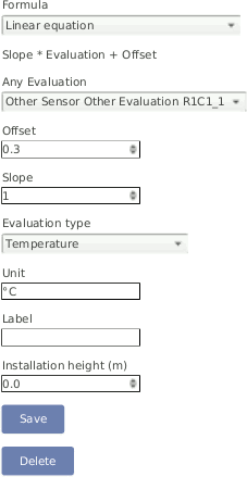
5.3.1.13. Linear equation

The linear equation can be used with any existing evaluation in order to apply an slope and offset. It can also be used to provide a dimensionless measurement (e.g. from a previously configured Other sensor) with a unit, an evaluation type, a height and a label for better interpretation.

Equation 5.19. Linear equation

A = Slope × B + Offset

Figure 5.7. Evaluation for linear equation

Screenshot of the Evaluation Configuration for Differential Temperature

5.3.1.14. Multiplication

Multiplication of two previously configured evaluations.

Equation 5.20. Multiplication

A = B × C

5.3.1.15. Turbulence intensity

Turbulence intensity (TI) is defined as the ratio of standard deviation of fluctuating wind velocity to the mean wind speed, and it represents the intensity of wind velocity fluctuation. It is calculated at the end of the averaging period (normally 10 minutes) and included in the measurement data CSV files.

Equation 5.21. Turbulence intensity

TI = σ(U) / avg(U)

where σ(U) is the standard deviation of the wind speed and avg(U) is the mean wind speed.

A commonly used procedure when analyzing turbulence data is to transform the horizontal wind vector in the geographical coordinate system into a rotated coordinate system that aligns with the mean wind direction during every averaging period. The longitudinal TI is defined as the standard deviation of longitudinal wind speed, normalized with the mean wind speed.

Equation 5.22. Longitudinal turbulence intensity

TI Long = σ(U) / avg(U)

where σ(U) is the standard deviation of the longitudinal wind speed and avg(U) is the mean wind speed.

5.3.1.16. Obukhov length

The Obukhov Length can be useful for turbulences analysis and is typically associated with a 3D ultrasonic sensor. To add this evaluation, the measurement of wind speed, wind direction, vertical wind speed and virtual temperature at one height are needed.

Equation 5.23. Calculation of the Obukhov Length

L = u_*³ / ( K × g / avg(T) × σ(V_Z, T))

Equation 5.24. Calculation of the friction velocity

u_* = (σ(V_X, V_Z)² + σ(V_Y, V_Z)²) ^1/4

where u_* is the friction velocity [m/s], g the gravitational acceleration 9.81[m/s²], σ(V_Z, T) the covariance of vertical wind speed and virtual temperature and K the von Kármán constant 0.41.

5.3.1.17. Obukhov stability parameter

Dimensionless stability parameter given by the normalized measuring height above ground z with the Obukhov length L. Can be useful for turbulences analysis and is typically associated with a 3D ultrasonic sensor. To add this evaluation, the measurement of wind speed, wind direction, vertical wind speed and virtual temperature at one height are needed.

Equation 5.25. Calculation of the Obukhov stability parameter

ζ = z / L

where z is the height above ground and L is the Obukhov length as in Section 5.3.1.16, “Obukhov length”.

5.3.1.18. Sensible heat flux

Sensible heat flux is measured with the eddy covariance method. In meteorology, it represents the heat exchanged between the Earth's surface and the atmosphere which resulted in a temperature change.

Equation 5.26. Calculation of the sensible heat flux

Q_H = ρ × C_p × σ(V_Z, T)

where ρ is the air density 1.2[kg/m ³], C _p the specific heat with constant pressure 1004.67[J/K/kg] and σ(V _Z, T) the covariance between the vertical wind speed and the temperature.

5.3.1.19. Solar zenith angle

The solar zenith angle is the angle between the zenith and the centre of the Sun's disc. It is calculated from the configured latitude and longitude and the time in the moment of the calculation.

	Important
	In order to use any formula based on the solar zenith angle, latitude and longitude of the measurement station have to be entered or acquired with a GPS device in the System → Administration menu (see also Section 4.2, “System Administration”).

5.3.1.20. Diffuse solar irradiance (DHI)

Equation 5.27. Calculation of Diffuse Solar Irradiance

DHI_[W/m²] = GHI_[W/m²] - DNI_[W/m²] × cos(θ)

where θ is the solar zenith angle.

	Note
	If the DNI pyranometer was tilted or not aligned to north, tilt angle and cardinal direction must be introduced. Tilt angle (°): (X axis) inclination angle with the Y axis aligned to north [-90°, 90°] Cardinal direction (°): Clockwise rotation from north around the Z axis [0°, 360°]

5.3.1.21. Total apparent power

Apparent power is the product of the rms (root mean square) values of voltage and current. It is taken into account when designing and operating power systems.

Equation 5.28. Calculation of total apparent power [S].

S_[VA] = U_1[V] × I_1[A] + U_2[V] × I_2[A] + U_3[V] × I_3[A]

5.3.1.22. Wind direction true-north

Combine the Kintech Geovane™ True-North direction with a measured wind direction at one-second level.

Equation 5.29. Calculation wind direction true-north.

Wind direction_{true-north[°]} = Wind direction_[°] - Offset_[°] + Direction_{true-north[°]}

Prev		Next
Chapter 4. System Configuration	Home	Chapter 6. Data Evaluation